


ABSTRACT
This paper reports on an update to the orbits and masses of the Martian satellites Phobos and Deimos. We obtained the orbits by fitting a numerical integration to all available Earth-based astrometry through the opposition of 2003, spacecraft imaging observations through 2007, and the Doppler tracking of the Viking and Phobos 2 spacecraft; the Doppler data provide information on the satellite masses. Our dynamical model included the figure acceleration due to a librating Phobos; we determined the amplitude of the forced libration. We also took into account the secular acceleration of Phobos due to the tide that it raises on Mars and estimated the Martian tidal quality factor Q. We provide an assessment of the accuracy of the orbits and a geometrical description of the orbits in the form of mean elements.
Export citation and abstract BibTeX RIS
1. INTRODUCTION
We developed our previous ephemerides of the Martian satellites (Jacobson et al. 1989) by fitting the Sinclair analytical theory (Sinclair 1972) to observations covering the period from 1877 to 1989. Later, we updated those ephemerides (Jacobson 1995) by incorporating theory improvements from Morley (1990) and additional observations made during the opposition of 1988 as well as imaging observations from the Phobos 2 spacecraft.
Since that update, we have received Earth-based astrometry from the U. S. Naval Observatory (USNO), Table Mountain Observatory (TMO), and the Laboratório Nacional de Astrofísica (LNA/MCT). We have also collected observations which were acquired by the Mars Global Surveyor (MGS) spacecraft with the Mars Orbiter Laser Altimeter (MOLA) instrument, by the Mars Express (MEX) spacecraft with the Super Resolution Channel (SRC) instrument, and by the Mars Reconnaissance Orbiter (MRO) spacecraft with the optical navigation camera. A fit of our theory to these new data together with the previous data did not produce a satisfactory result. We concluded that the theory is not sufficiently complete to accommodate the recent high precision spacecraft data. Rather than attempting to improve the theory, we opted to fit numerically integrated orbits to the observations; a fit of integrated orbits to all but the TMO, LNA/MCT, MRO, and latest MEX data has already been carried out by Lainey et al. (2007).
Because we are using a numerically integrated dynamical model for the satellite orbits, we augmented our data set with tracking data from the Viking 1 and Viking 2 spacecraft (Snyder 1977, 1979) and the Phobos 2 spacecraft (Sagdeev & Zakharov 1989). These data have been used by a number of investigators to determine the satellite GMs. Rather than relying on one of those earlier sets of GMs, we decided to estimate the GMs directly in our orbit fit. Unfortunately, the coverage of the tracking data is insufficient to permit the estimation of parameters in extended gravity fields for the satellites.
2. DYNAMICAL MODEL
2.1. Satellite Orbits
The model for the satellite orbits is a numerical integration of their equations of motion (Peters 1981). The formulation is in Cartesian coordinates centered at the Martian system barycenter and referenced to the International Celestial Reference Frame (ICRF). The modeled dynamics include the asphericity of Mars, the mutual interactions of Phobos and Deimos, the perturbations due to the Earth, Moon, Jupiter, Saturn, and the Sun, the Phobos figure, and the tide raised on Mars by Phobos. We ignore the tide raised by Deimos; because of Deimos's smaller mass and larger distance from Mars, the tidal acceleration caused by Deimos is roughly 3 orders of magnitude smaller than that caused by Phobos. Moreover, to date there has been no conclusive observational evidence of a tidal effect on Deimos. We do, however, account for the effect of the tide due to Phobos on the motion of Deimos (our software applies active tidal forces to all bodies being integrated). In modeling the acceleration induced by the Phobos figure, we assume that Phobos is in synchronous rotation with its pole normal to its orbit plane and its prime meridian librating about the sub-Mars direction (i.e., a libration in longitude); the libration in latitude is ignored.
JPL planetary ephemeris DE421 (Folkner et al. 2008) provides the positions and GMs of the Sun, Moon, and planets. The Love number, gravity field, and orientation of Mars are from Konopliv et al. (2006). We truncated the gravity field at degree 8 in the zonal harmonics and fifth degree and order in the tesseral harmonics; tests showed higher degree and order had only meter level effects on the integration. Because of software limitations, we could not use the Mars orientation model as published. Instead, we fit a Fourier series to the ICRF pole right ascension and declination and the prime meridian derived from the model. The series, given in the Appendix, reproduces the angles at the 6 mas level which is well below their actual uncertainty. The Phobos quadrupole field gravitational harmonics (J2 and C22) in the figure acceleration are from Borderies & Yoder (1990).
2.2. Spacecraft Orbits
In order to process the Viking and Phobos 2 tracking data, we also had to model the spacecraft orbits. These orbits are numerically integrated with JPL's Orbit Determination Program (ODP; Moyer 1971; Ekelund 1979), which is the software set used at JPL for planetary spacecraft navigation. Like the satellite orbits, the spacecraft orbits are represented by Cartesian coordinates centered at the Martian system barycenter and referenced to the ICRF. The gravitational model for the spacecraft is the same as that for the satellites except we did not truncate the Mars gravity field or approximate the Mars orientation (the published gravity field and orientation model are designed to be used in the ODP). We ignored the effect of the Phobos tide on the spacecraft but included the Phobos figure acceleration, i.e., Phobos was not treated as a point mass during the spacecraft flybys. Because the flybys are close to Phobos, the Phobos figure causes a small disturbance in the spacecraft orbits; the figure effect is small enough that could have been neglected, but we retained it for dynamical completeness.
All three spacecraft were affected by the force due to solar radiation pressure. We accounted for this force with a simple bus model characterized by effective areas along and normal to the spacecraft–Sun direction. The spacecraft were three-axis stabilized, i.e., their orientation was changed and maintained by attitude control thrusters. Consequently, their motion was subject to small accelerations due to thruster imbalances and control system leakage; we included those effects in our force model as small accelerations along the spacecraft body axes. We have no detailed history of the actual attitudes of the spacecraft body axes. However, we know that the Viking axis of symmetry was normally directed toward the Sun, and the other two axes were set with the aid of a reference star. Phobos 2 was also oriented relative to the Sun and stars. For modeling purposes, we adopted the spacecraft–Sun direction as one body axis for all three spacecraft. The direction to the star Canopus defined the roll angle about that axis.
On 1989 March 25, Phobos 2 was reoriented in order to take pictures of Phobos (the camera was fixed to the spacecraft which necessitated turning it to point the camera). The disturbances induced by the turns were modeled as an impulsive maneuver on that date.
3. OBSERVATIONS
Morley (1989) published a catalog of astrometric observations for the period 1877–1982 as the source of Earth-based data for the improvement of the satellite ephemerides supporting the Phobos 2 mission. The oppositions of 1986 and 1988 provided additional observations (Kiseleva & Chanturiia 1988; Kiselev et al. 1989; Jones et al. 1989; Shor 1989; Kalinichenko et al. 1990; Tel'nyuk-Adamchuk et al. 1990; Bobylev et al. 1991; Nikonov et al. 1991; Colas 1992; Kudryavtsev et al. 1992). V. Golovnya (2001, private communication) collected a catalog of observations for the period 1963–1988 made at the Golosseevo-Kiev, Kitab, and Shokin Majdanak observatories; many of these are a modern re-reduction of observations given by Morley. Between 1967 and 2003, a significant series of observations were made at the USNO (D. Pascu 1988 & 2003, private communication). In 1995, CCD observations of Deimos were made at LNA/MCT followed in 2003 by Phobos and Deimos observations (Veiga 2008). W. M. Owen (2003, private communication) also observed both satellites from TMO.
In 1971, the first spacecraft imaging observations were made by Mariner 9 (Duxbury & Callahan 1989). Subsequently, there has been imaging during 1976–1980 by the two Viking spacecraft (Duxbury & Callahan 1988), in 1989 by Phobos 2 (Kolyuka et al. 1991), in 1998 by MGS (C. E. Hildebrand 1998, private communication), in 2006 by MRO (S. P. Synnott 2006, private communication), and between 2004 and 2007 by MEX (Oberst et al. 2006; Willner et al. 2008). With the exception of MRO, the observations are in the form of astrometric positions of the satellite as seen from the spacecraft. The MRO data are the line and sample location of the satellite image recorded by the spacecraft camera against a star background (the stars define the orientation of the camera).
In 1998, transit observations of the shadow of Phobos on Mars were acquired with the MOLA instrument on MGS; Bills et al. (2005) converted them into positions of Phobos as seen from Mars.
Most of the observations are available from the Natural Satellites Data Center (NSDC) which is maintained as a collaborative effort by the Institut de Mécanique Céleste et de Calcul des Ephémérides (IMCCE) in Paris, France1 and the Sternberg Astronomical Institute (SAI) at the Moscow University, Russia2 (Arlot & Emelyanov 2009).
The Viking tracking data are two-way coherent S-band Doppler acquired at the Deep Space Network (DSN) sites at Goldstone, California; Madrid, Spain; and Canberra, Australia. They are the same data used by Konopliv et al. (2006) for his satellite GM determination in connection with his Mars gravity field development. The Viking 1 data cover the period from 1977 February 8 to 1977 March 7 when the spacecraft was on a trajectory designed to provide close-up photography of Phobos and close flybys to support a GM estimate; there were 29 flybys at distances ranging from 800 km to 97 km. The tracking period for Viking 2 is 1977 October 15 to 1977 October 17; the spacecraft made a single close approach to Deimos on October 15 at a distance of 31 km.
The Phobos 2 tracking data consist of 15 passes of C-band range rates measured at the Evpatoria and Ussuriysk tracking stations in Russia from 1989 March 21 to 1989 March 27 (V. Stepanyants 2008, private communication). These passes were of short duration, about 10 minutes, because of thermal limitations of the transmitters. During tracking time frame, Phobos 2 was in a quasi-synchronous orbit (QSO) with respect to Phobos; the spacecraft's and satellite's orbital periods and planes were nearly coincident but their eccentricities differed slightly. Consequently, the spacecraft motion relative to Phobos appeared nearly elliptical with the distance to Phobos ranging between 185 and 400 km.
We calibrated all of the tracking data for ionosphere delays with corrections derived from the Bent model, a global empirical ionospheric model that gives the electron density profile as a function of latitude, longitude, time of day, season, and solar flux (Bent et al. 1976). For the Viking data, we applied the standard DSN seasonal troposphere calibrations (Chao 1971). Since no analogous troposphere adjustments were available for the Phobos 2 data, we assumed a zenith delay of 210 cm, a typical value that should be accurate to about 10%.
4. ANALYSIS
4.1. Solution Method
We fit the orbits, in a weighted least-squares sense, to the observational data by adjusting the values of the parameters in our dynamical and observational models. The dynamical parameters are: (1) the epoch position, velocity, and GM of each satellite, (2) the amplitude of the Phobos longitude libration (see Section 4.3), (3) the Phobos tidal bulge lag angle (see Section 4.4), (4) the epoch states, solar pressure coefficients, and non-gravitational accelerations for the Viking and Phobos 2 spacecraft, and (5) the Phobos 2 impulsive maneuver.
The observational model parameters are as follows.
- 1.
- 2.Adjustments to the Mariner 9, Viking, and Phobos 2 trajectories associated with the respective imaging data; for the Mariner 9 imaging acquired on the approach to Mars, we corrected the direction of the spacecraft's trajectory (i.e., the inertial direction of the asymptote of the hyperbolic conic approximation to the trajectory); for the Mariner 9, Viking, and Phobos 2 imaging acquired in orbit about Mars, we corrected the spacecraft orbit node on the plane normal to the Earth–Mars line of sight; for the Viking and Phobos 2 imaging, we also corrected the time of spacecraft orbit periapsis passage. See Duxbury & Callahan (1988, 1989) and Kolyuka et al. (1991) for details on the spacecraft orbit adjustment procedures.
- 3.The camera pointing angles and satellite image phase biases for the MRO data, the known locations of background stars in the pictures specify the camera pointing, the image phase biases account for lighting effects which introduce errors in the determination of the center of figure of the extended satellite images. The phase biases are directed toward the Sun with magnitude a bjsinj(ϕ/2) where a is the radius of the satellite, bj is the estimated phase bias scale factor, and ϕ is the solar phase angle. We included the three bias terms for j = 0, 1, 2.
- 4.Corrections to the spacecraft tracking data ionosphere calibrations to account for inaccuracies in the delays computed from Bent model discussed in the previous section.
- 5.Corrections to the spacecraft tracking data troposphere calibrations to account for the daily variations in troposphere delay.
- 6.
- 7.The tracking station locations associated with the Phobos 2 data; the station locations contained small systematic errors because the data used to determine them were not completely calibrated (Kroger et al. 1992).
We were unable to determine the Phobos J2 and C22 as part of our orbit fit and conclude that there is insufficient information in the data set to isolate these parameters.
We grouped the Earth-based astrometric data according to type, observatory, and the observing period in which they were acquired. Data weights for each group were assigned through an iterative process to be consistent with the root mean square (rms) of the residuals (the differences between the actual observations and their values predicted by our model) of that group. Analogous to the Earth-based astrometry, the MGS, MRO, and MEX spacecraft imaging data and MOLA transit data were given weights consistent with the rms of their respective residuals.
For the imaging observations from Viking and Phobos 2, we initially tried the weights suggested in the publications. However, after looking at the residuals we concluded that the weights were too pessimistic. Ultimately, we tightened the Viking 1 weights by 75%, the Viking 2 weights by 65%, and those for Phobos 2 by 85%.
We based the Viking Doppler data weights for each tracking pass on the rms of the residuals for that pass scaled by a factor to account for the fact that the Doppler noise is not a white-noise process (Folkner 1994). The scale factor is 0.468(86400/τ)1/3 where τ is the Doppler sample interval in seconds (for a 10 minute sample interval the factor is 2.45). This scaling preferentially weights the Doppler at the diurnal frequency (86,400 s); however, it yields a weight which is too conservative for the satellite close encounter data. For the Phobos and Deimos encounter passes, we employed the weighting algorithm (Mackenzie & Folkner 2006) which was developed for Cassini planetary gravity analysis; the same algorithm was applied to all of the short duration Phobos 2 tracking passes as well. The algorithm accounts for the noise structure of the tracking data, but it is designed for short arcs of tracking data where the characteristic signature in the data is that of the gravity parameters in a close planet or satellite flyby.
To fit the weighted observations, we used a batch-sequential square-root information filter with a number of parameters treated as white-noise stochastic parameters, i.e., parameters which are constant within a batch but vary from batch to batch. See Bierman (1977) for a discussion of square-root information filtering. Our stochastic parameters were: (1) Colas's CCD scale and orientation batched according to observation series (Colas & Arlot 1991); (2) the Mariner 9, Viking, and Phobos 2 orbit node batched by orbit about Mars; (3) the Viking and Phobos 2 periapsis timing batched by orbit about Mars; (4) the MRO camera pointing angle batched by picture; (5) the spacecraft tracking data ionosphere and troposphere calibration corrections batched by day; (6) the Viking Doppler biases batched by tracking pass; and (7) the spacecraft non-gravitational accelerations batched by the times of Mars periapsis and apoapsis for Viking 1 and Phobos 2 and the times of apoapsis for Viking 2.
Table 1 gives the postfit residual statistics for the observations grouped by source (although the original source is provided, most of the pre-1982 observations appear in Morley's catalog). For those observations which were made in the form of position angles, we scaled the residuals by the separation distance before forming the rms. The residuals for spacecraft based data were converted to units of km depending upon the spacecraft satellite range at time of the measurement. For the purpose of comparison, the Earth-based astrometry can be converted to km with the factor 375 km arcsec−1. Examination of the statistics shows that the best Earth-based astrometry (Veiga 2008) fits to the 19 km level and the best spacecraft imaging (Willner et al. 2008) fits to the 0.5 km level. Although the statistics cannot be compared directly to those in Table 3 in Jacobson et al. (1989) which groups the rms by opposition rather than source, we have verified that for the pre-1988 data our new orbits provide a fit comparable to our previous orbits.
Table 1. Observation Residual Statistics
| Source | Number | rms | ||||
|---|---|---|---|---|---|---|
| Pho. | Dei. | D-P | Pho. | Dei. | D-P | |
| Hall (1878) | 79 | 108 | 0 782 782 |
0742 |
||
| Pickering (1882) | 110 | 290 | 0753 |
0825 |
||
| Pritchett (1878) | 11 | 11 | 0713 |
1031 |
||
| Common (1878) | 23 | 1069 |
||||
| Christie et al. (1878) | 6 | 0839 |
||||
| Hall (1880) | 81 | 90 | 0337 |
0521 |
||
| Pritchett (1880) | 10 | 5 | 1113 |
1181 |
||
| Common (1879) | 43 | 60 | 0875 |
0880 |
||
| Lindsay (1879) | 19 | 0855 |
||||
| Pritchard (1880) | 10 | 0566 |
||||
| Maunder (1880) | 8 | 0862 |
||||
| Hall (1882) | 13 | 21 | 0523 |
0584 |
||
| Common (1882) | 9 | 10 | 0577 |
0908 |
||
| Hall (1884) | 4 | 19 | 0819 |
0531 |
||
| Brown (1891) | 10 | 0621 |
||||
| Keeler (1888) | 115 | 52 | 1 | 0398 |
0610 |
0430 |
| Hall (1888) | 4 | 21 | 0483 |
0561 |
||
| Keeler (1890) | 47 | 26 | 0310 |
0590 |
||
| Hall (1891) | 9 | 12 | 0684 |
0975 |
||
| Campbell (1892) | 93 | 87 | 0405 |
0517 |
||
| Hall (1893) | 35 | 37 | 0714 |
0956 |
||
| Campbell (1895) | 398 | 345 | 0253 |
0299 |
||
| Newall (1895) | 77 | 0644 |
||||
| Barnard (1897) | 113 | 30 | 0423 |
0479 |
||
| Schaeberle (1897) | 51 | 65 | 0430 |
0618 |
||
| Kostinsky (1897) | 4 | 0222 |
||||
| Hussey (1898) | 60 | 20 | 0276 |
1114 |
||
| Struve (1898) | 79 | 76 | 1 | 0226 |
0506 |
0200 |
| Wirtz (1909) | 4 | 10 | 0668 |
0720 |
||
| USNO (1911) | 97 | 137 | 0384 |
0513 |
||
| Aitken (1909) | 48 | 40 | 0308 |
0330 |
||
| Barnard (1910) | 14 | 13 | 0304 |
0214 |
||
| Wirtz (1912) | 8 | 10 | 6 | 0448 |
0759 |
0393 |
| Kostinsky (1913) | 48 | 40 | 0591 |
0739 |
||
| USNO (1929) | 416 | 377 | 0407 |
0431 |
||
| Jeffers (1925) | 101 | 70 | 0362 |
0388 |
||
| USNO (1954) | 50 | 26 | 43 | 0432 |
0536 |
0242 |
| Rizvanov & Shshukin (1969) | 22 | 0770 |
||||
| Karimova & Kholopov (1969) | 4 | 0588 |
||||
| Kovalenko (1969) | 7 | 1035 |
||||
| Fatchikhin (1970) | 63 | 0769 |
||||
| Deutsch (1970) | 8 | 52 | 0489 |
0691 |
||
| Bashtova & Rakhimov (1973) | 21 | 0985 |
||||
| Khatisov & Salukvadze (1974) | 39 | 44 | 0731 |
0721 |
||
| Khatisov & Salukvadze (1975) | 118 | 228 | 0542 |
0569 |
||
| Kovalenko et al. (1980) | 26 | 90 | 0848 |
0690 |
||
| van Biesbroeck (1970) | 44 | 0325 | ||||
| Kiseleva (1976) | 34 | 0437 | ||||
| Tolbin (1985) | 12 | 26 | 0850 |
0614 |
||
| A. T. Sinclair (1988, private communication) | 22 | 0533 | ||||
| Kiseleva & Chanturiia (1988) | 12 | 0609 |
||||
| Duxbury & Callahan (1988) | 326 | 212 | 8.54 km | 4.00 km | ||
| D. Pascu (1988, private communication) | 302 | 420 | 112 | 0156 |
0165 |
0200 |
| Duxbury & Callahan (1989) | 102 | 62 | 10.85 km | 10.84 km | ||
| Kiselev et al. (1989) | 224 | 100 | 0908 |
0745 | ||
| Jones et al. (1989) | 172 | 24 | 126 | 0134 |
0137 |
0183 |
| Shor (1989) | 280 | 160 | 213 | 1111 |
1020 |
0567 |
| Kalinichenko et al. (1990) | 28 | 2 | 28 | 0321 |
0096 |
0119 |
| Tel'nyuk-Adamchuk et al. (1990) | 190 | 88 | 56 | 0942 |
1084 |
0774 |
| Bobylev et al. (1991) | 324 | 104 | 276 | 0486 |
0668 |
0418 |
| Nikonov et al. (1991) | 46 | 0530 |
||||
| Kolyuka et al. (1991) | 74 | 14 | 0.65 km | 9.93 km | ||
| Colas (1992) | 1626 | 0243 | ||||
| Kudryavtsev et al. (1992) | 1198 | 0118 | ||||
| C. E. Hildebrand (1998, private communication) | 4 | 3.06 km | ||||
| V. Golovnya (2001, private communication) | 72 | 349 | 188 | 0879 |
0779 |
0473 |
| W. M. Owen (2003, private communication) | 6 | 12 | 0224 |
0169 | ||
| D. Pascu (2004, private communication) | 14 | 10 | 414 | 0379 |
0219 |
0062 |
| Bills et al. (2005) | 32 | 2.72 km | ||||
| Oberst et al. (2006) | 52 | 20 | 1.64 km | 4.90 km | ||
| S. P. Synnott (2006, private communication) | 103 | 478 | 6.96 km | 5.33 km | ||
| Veiga (2008) | 282 | 304 | 0056 |
0051 |
||
| Willner et al. (2008) | 138 | 0.49 km | ||||
Figures 1–3 display the residuals for the respective Viking 1, Viking 2, and Phobos 2 Doppler tracking. No obvious signatures remain, and the scatter is reasonable for S-band and C-band tracking. The apparent noise increase at the Deimos encounter (1977 October 15, 11:15:00) is a consequence of the reduction of the Doppler sample interval from 1 minute to 10 s.

Figure 1. Viking 1 Doppler residuals.
Download figure:
Standard image High-resolution image
Figure 2. Viking 2 Doppler residuals.
Download figure:
Standard image High-resolution image
Figure 3. Phobos 2 Doppler residuals.
Download figure:
Standard image High-resolution imageTable 2 contains the epoch state vectors determined from the fit; the vector components are specified to sixteen digits to facilitate future orbit integrations.
Table 2. Barycentric State Vectors at 1976 July 24 (TDB)
| Satellite | Position (km) | Velocity (km s−1) |
|---|---|---|
| Phobos | −7250.412601711135 | 0.9988670536572896 |
| −5870.213549601684 | −1.3800306900339470 | |
| 898.4275832484670 | −1.2924979187687260 | |
| Deimos | 14750.74693771948 | −0.8968342728440282 |
| 18168.22949466721 | 0.6580512035236056 | |
| 1647.735099652305 | 0.7669278908791312 |
Note. The timescale for JPL ephemerides is Temps Dynamique Barycentrique, Barycentric Dynamical Time (TDB; IAU 2006).
Download table as: ASCIITypeset image
4.2. Satellite GMs
Table 3 summarizes a number of previous determinations of the satellite GMs together with our results.
Table 3. Satellite GMs km3 s−2×10⁻⁴
| Reference | Phobos | Deimos |
|---|---|---|
| Christensen et al. (1977) | 6.6± 0.8 | |
| Tolson et al. (1977) | 7.3± 0.7 | |
| Hildebrand et al. (1979) | 1.7± 2.2 | |
| Williams et al. (1988) | 8.5± 0.7 | 1.2± 0.1 |
| Berthias (1990) | 7.163± 0.008 | |
| Kolyuka et al. (1990) | 7.22± 0.05 | |
| Smith et al. (1995) | 5.87± 0.03 | 0.91± 0.55 |
| Konopliv et al. (2006) | 7.160± 0.005 | 0.98± 0.07 |
| Shishov (2008) | 7.158± 0.001 | |
| Rosenblatt et al. (2008a) | 7.11± 0.02 | 1.0± 0.6 |
| Andert et al. (2008) | 7.09± 0.02 | |
| Rosenblatt et al. (2008b) | 7.15± 0.02 | 1.12± 0.5 |
| Viking only (no nongrav) | 7.077± 0.003 | 1.02± 0.02 |
| Viking only | 7.126± 0.045 | 1.01± 0.03 |
| Phobos 2 only (no nongrav) | 7.090± 0.004 | |
| Phobos 2 only | 7.091± 0.005 | |
| Viking+Phobos 2 | 7.092± 0.004 | 1.01± 0.03 |
Download table as: ASCIITypeset image
The first estimates of the Phobos GM using Viking 1 tracking data were by Christensen et al. (1977), who deduced the GM from the changes in the mean orbital period of the spacecraft caused by 14 consecutive close Phobos flybys, and by Tolson et al. (1977), who fit the spacecraft orbit and the GM directly to the data from the three closest spacecraft flybys. Hildebrand et al. (1979) made the initial Deimos GM estimate with 1 hr of tracking acquired during the Viking 2 flyby. Williams et al. (1988) later obtained both GMs using the combined tracking from 8 Viking 1 Phobos flybys and the Viking 2 Deimos flyby. Konopliv et al. (2006) found the GMs as part of his determination of the Martian gravity field by including data from 29 Viking 1 Phobos flybys and the Viking 2 Deimos flyby.
Berthias (1990) estimated the Phobos GM in a fit to the Phobos 2 tracking data over the period 1989 February 18 to 1989 March 27; he also estimated the spacecraft orbit, maneuvers, and the Phobos ephemeris. Kolyuka et al. (1990) carried out a similar fit but restricted his data span to the period of the QSO. Shishov (2008) processed the tracking data within the context of his development of a numerically integrated Phobos ephemeris.
Smith et al. (1995) took a different approach to the use of spacecraft tracking; they inferred the satellite GMs from the satellites' contribution to the long period secular perturbations of the Mariner 9 and Viking spacecraft orbits.
Rosenblatt et al. (2008a) applied the same approach as Smith et al. (1995) but to the MEX spacecraft which, because of its orbital geometry, was more sensitive to the satellite perturbations. Rosenblatt et al. (2008b) later extended that analysis by adding the tracking data from a close Phobos flyby by MEX. Andert et al. (2008) obtained their result with the MEX tracking from two close flybys of Phobos.
Our Deimos GM is in agreement with all previous results. Its uncertainty is smaller than those associated with the earlier determinations from the Viking 2 tracking, most likely a consequence of our data weighting strategy. The values found from the MEX data are a good match for those based on the Viking 2 data but are considerably less well determined because MEX has had no close Deimos flybys.
There is considerable variation among the various Phobos GMs. This is not too surprising because, unlike with Deimos, data from multiple satellite flybys contribute to the Phobos GM determination. Consequently, dynamical modeling of both the spacecraft and satellite motions have a significant effect on the result. All of the pre-2006 work employed Mars gravity fields derived from Mariner 9 and Viking data (Gapcynski et al. 1977; Christensen & Balimino 1979). The analysis by Shishov (2008) used the field of Lemoine et al. (2001) based on MGS data, and the remaining post-2006 work relied on the field of Konopliv et al. (2006). Prior to 2008, the orbit of Phobos was represented by analytical theories (Sinclair 1972; Born & Duxbury 1975; Ivanov et al. 1988; Morley 1990; Chapront-Touzé 1990). Tolson et al. (1977), however, fit a numerical integration to the Born–Duxbury theory and used the integrated orbit when processing the spacecraft tracking. For the analysis of the MEX tracking, Rosenblatt et al. (2008a, 2008b) took the integrated ephemeris of Lainey et al. (2007) whereas Andert et al. (2008) chose the integrated ephemeris of Jacobson (2008). As stated earlier, Shishov (2008) has developed his own integrated orbit.
All previous investigators allowed for solar radiation pressure on the various spacecraft. However, in work involving either the Phobos 2 or Viking data, only Kolyuka et al. (1990) and Konopliv et al. (2006) considered the effects of unmodeled non-gravitational accelerations. The former found the accelerations on Phobos 2 to be negligible, and the latter added small impulsive maneuvers to his Viking data processing to account for unmodeled forces. Table 3 contains our GM values based on only the Viking tracking and only the Phobos 2 tracking for cases in which those accelerations were either excluded or included. It is clear that the accelerations have little effect on Phobos 2 but have a major effect on Viking 1. Ignoring the Viking 1 accelerations yields a Phobos GM closer to the value found with the Phobos 2 data alone and drastically reduces the uncertainty. Accounting for the accelerations leads to an increase in both the value and uncertainty; however, a statistical agreement remains between the two single spacecraft determinations. The GM found with the combined data set, our adopted value, is essentially the same as that found with the Phobos 2 data because the strength of the Viking 1 data is significantly weakened by the non-gravitational accelerations.
4.3. Phobos Figure Acceleration and Libration
Under our assumptions that Phobos is in synchronous rotation with its pole normal to its orbit plane and its axis of minimum principal moment of inertia directed toward Mars, the potential for the acceleration of Mars due to the Phobos quadrupole gravity field is:
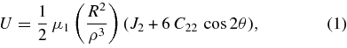
where
μ1 = GM of Phobos,
R = equatorial radius of Phobos,
ρ = distance from Phobos to Mars,
J2 = second degree zonal harmonic of Phobos,
C22 = second degree and order tesseral harmonic of Phobos, and
θ = the angle between the direction from Phobos to Mars and the axis of minimum principal moment of inertia.
Because Phobos's rotation rate matches the orbit's mean longitude rate (synchronous rotation), and because Phobos is assumed to librate about the sub-Mars direction:

where f is the true anomaly, M is the mean anomaly, and τ is the forced libration angle. The Phobos-forced libration takes the form (Duxbury 1977):

From the elliptic expansion of true anomaly in terms of mean anomaly:

where e is Phobos's orbital eccentricity.
In our numerical integration, we compute the force on the planet exerted by Phobos based on the potential (Equation (1)) and the libration angle (Equation (4)):
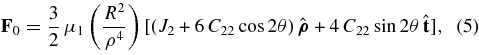
where  is the unit vector directed from Mars toward Phobos and
  is the unit vector in the Phobos orbit plane normal to
  and in the direction of Phobos's orbital motion. The reactive force acting on Phobos is
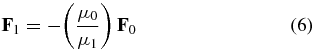
with μ0 being the GM of Mars. This force introduces both secular and periodic perturbations into Phobos's orbit.
We can ascertain the nature of the perturbations by applying Lagrange's planetary equations to disturbing function, Equation (1), to obtain approximate analytical expressions for the perturbations in Phobos's orbital elements:
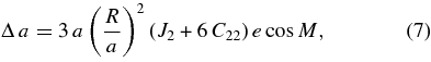
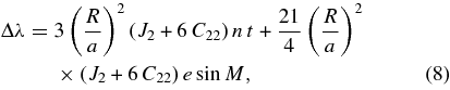
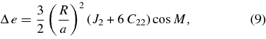
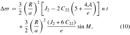
where a is the semi-major axis, λ is the mean longitude, ϖ is the longitude of periapsis, n is the mean motion, and t is time from epoch. Because our force has no component normal to the orbit plane, it has no effect on the orbital inclination or longitude of ascending node. Note that only the ϖ secular rate depends on the forced libration. We find that the amplitudes of the periodic terms for a and λ are sub-meter; the e amplitude is about 4 m, and that for ϖ is about 270 m. The secular rates are about 0.35 deg yr−1 and 0.19 deg yr−1 for the mean longitude and periapsis longitude, respectively.
Table 4 contains our estimated Phobos-forced libration amplitude. For comparison purposes, the table includes the libration amplitude observed optically from Viking 1 images by Duxbury & Callahan (1989) and the amplitude and periapsis rate from the analytical work of Borderies & Yoder (1990). The agreement among the amplitudes lends credence to our result. Yet, we emphasize that our determination of  is indirect, dependent upon our total force model and the postulated Phobos gravity field. If we assume, as suggested by Equations (7)–(10), that the only observable effect of the libration on the orbit is its contribution to the periapsis precession, then we are implicitly finding
  from the difference between the total observed precession and that produced by the Mars gravity field and the solar and planetary perturbations.
Table 4. Phobos Figure Parameters
| Reference |  |
 |
|---|---|---|
| (deg) | (deg yr−1) | |
| Duxbury & Callahan (1989) | 0.81± 0.5 | |
| Borderies & Yoder (1990) | 1.19 | −0.18 |
| Current | 1.03± 0.22 | −0.19 |
Download table as: ASCIITypeset image
Equation 10 also provides some insight into the difficulty in determining the Phobos gravitational harmonics from the data fit. Again, if we assume that the only observable effect of the figure acceleration is the periapsis precession, it is clear that only one of the three parameters from  , and
, and  can be independently estimated from the observed
  .
.
4.4. Phobos Secular Acceleration and the Tidal Q of Mars
By analyzing the observed longitudes of Phobos between 1877 and 1941, Sharpless (1945) discovered the secular acceleration in its mean longitude. All of the theories of the satellite's motion developed subsequently have included the acceleration. Table 5 provides the accelerations, s, from a sampling of the theories which have been fit to observations.
Table 5. Phobos Secular Acceleration and Mars Tidal Parameters
| Reference | s × 10−3 | κ2 | Q | γ |
|---|---|---|---|---|
| (deg yr−2) | (deg) | |||
| Sharpless (1945) | 1.882± 0.171 | |||
| Shor (1975) | 1.427± 0.147 | |||
| Sinclair (1978) | 1.326± 0.118 | |||
| Jacobson et al. (1989) | 1.249± 0.018 | |||
| Chapront-Touzé (1990) | 1.270± 0.008 | |||
| Emelyanov et al. (1993) | 1.290± 0.010 | |||
| Bills et al. (2005) | 1.367± 0.006 | 0.163 | 85.6± 0.4 | 0 3346± 00014 3346± 00014 |
| Rainey & Aharonson (2006) | 1.334± 0.006 | 0.153 | 78.6± 0.8 | 03645± 00039 |
| Lainey et al. (2007) | 1.270± 0.015 | 0.152 | 79.9± 0.7 | 03585± 00031 |
| Current | 1.270± 0.003 | 0.152 | 82.8± 0.2 | 03458± 00009 |
Download table as: ASCIITypeset image
It is generally agreed that the cause of the acceleration is the force due to the tide raised on Mars by Phobos. Bills et al. (2005) deduced the acceleration from fit of a quadratic polynomial to the observed Phobos longitudes over the 1877–2004 time frame and computed the tidal lag angle, γ, in an analytical model of a tidally induced acceleration (Redmond & Fish 1964). The lag angle is the angle between the Mars centered position of the tidal bulge and the position at which the tide acts. The tidal quality factor, Q, is related to the lag: Q = cot 2γ. Rainey & Aharonson (2006) extended the work of Bills et al. by incorporating high accuracy observations of the Phobos shadow on Mars made with the Mars Orbiter Camera on MGS. The accelerations and tide parameters from these two analyses appear in Table 5.
In our numerical integration, we modeled the tide raised by Phobos at position ρ* relative to Mars, the position of the tidal bulge, with a second-order potential that acts at position ρ (Mignard 1979):
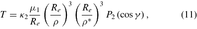
where
κ2 = the Love number of Mars,
μ1 = GM of Phobos,
Re = the equatorial radius of Mars,
ρ = the magnitude of  ,
,
ρ* = the magnitude of  ,
,
P2 = the Legendre polynomial of degree 2, and
γ = the angle between  and
and  .
.
Lainey et al. (2007) employed a similar model in their integration. Table 5 gives our results together with theirs; in our fit we estimated γ whereas they estimated Q. The accelerations match but we differ in the tidal parameters primarily because we used different values for μ1.
There is actually pretty good agreement among the accelerations estimated in data fits with both theories and integrations; the result from the high precision theory of Chapront-Touzé (1990) is identical to that from the integrations. The accelerations found from examining only the longitudes (Sharpless 1945; Bills et al. 2005; Rainey & Aharonson 2006) are all larger than the accelerations from the data fits.
5. COMPARISON WITH PREVIOUS ORBITS
Figures 4 and 5 compare our current Phobos and Deimos orbits with our previously published orbits (Jacobson et al. 1989) in terms of differences in the radial direction from the planet, the transverse (normal to the radius) direction, and the direction normal to the orbit plane. The slopes in the transverse direction indicate changes in the mean motions, and the slight curvature is a consequence of secular acceleration differences; the earlier Deimos orbit had a secular acceleration, the current orbit does not. The expanding envelopes in the radial and normal directions reflect changes in the periapsis and nodal precession rates. Because of its small eccentricity, periapsis precession rate differences have little effect on Deimos. It is clear from the figures that an update to our orbits was sorely needed.
Figure 4. Phobos orbit comparison with previous JPL.
Download figure:
Standard image High-resolution image
Figure 5. Deimos orbit comparison with previous JPL.
Download figure:
Standard image High-resolution imageFigures 6 and 7 show the differences between our orbits and those of Lainey et al. (2007). We are in quite good agreement with respect to Phobos. The slight mean motion difference can be attributed to the high accuracy observations of Veiga (2008) and Willner et al. (2008) which were unavailable to Lainey et al. (2007). We have a significant disagreement in the mean motion of Deimos; it is probably caused by our use of the Veiga's astrometry and the MRO imaging.

Figure 6. Phobos orbit comparison with Lainey.
Download figure:
Standard image High-resolution image
Figure 7. Deimos orbit comparison with Lainey.
Download figure:
Standard image High-resolution image6. ACCURACY OF THE ORBITS
One measure of the accuracy of the orbits is the solution formal covariance. However, that measure is normally optimistic because the formal covariance does not account for systematic or unmodeled errors in the orbit or observation modeling or in the observations themselves. Because our models are quite detailed and can be fit to the observations at their presumed accuracies, we believe any significant systematic errors are most likely in the observations. By including observation biases as "consider" parameters in our estimation process, we introduced some additional uncertainty due to observational error. Consider parameters are parameters which are not estimated but whose uncertainty contributes to the uncertainty in the estimated parameters (Bierman 1977). We based the values of the bias uncertainties on the observation residuals for the various observation sets. The uncertainties varied from roughly 300 mas for some of the old photographic position observations to 10 mas for recent CCD positions. The old visual micrometer measures were assumed to be biased at about the 50 mas level.
Figures 8 and 9 display the orbit uncertainties from the consider covariance mapped into the radial, transverse, and out-of-plane directions over a twenty-year time period (the units are meters for Phobos and kilometers for Deimos). As with most satellite orbits, the transverse uncertainties grow due to the uncertainties in the orbital mean motion. Phobos, however, has additional growth caused by the error in the tidal acceleration, as seen by the slight bend in Figure 8(a).
Figure 8. Phobos orbit uncertainties.
Download figure:
Standard image High-resolution image
Figure 9. Deimos orbit uncertainties.
Download figure:
Standard image High-resolution image
Another assessment of accuracy can be made by comparing results obtained with different data sets and processing procedures. For example, our current orbits match those from Jacobson (2007) at the 3–4 km level (transverse direction) for both satellites. But that earlier solution did not model the Phobos libration, used the satellite GMs from Konopliv et al. (2006), and did not fit the observations from Veiga (2008) or Willner et al. (2008). The orbits from Jacobson (2008, 2009) agree with the current ones at 1–2 km level for Phobos and the 2–3 km level for Deimos. Those analyses fit the current observation set with the current satellite orbit modeling but with slightly different spacecraft modeling and processing of the spacecraft tracking data. The spacecraft body axes were defined with the Viking roll axes directed toward Mars and the Phobos 2 roll axis directed toward Phobos; the Y-axes were along the vector product of Mars relative velocity and the roll axes, and the X-axes completed a right-handed system. For Phobos 2, only one rather than all three of the bus model solar pressure coefficients was estimated. In addition, the non-gravitational accelerations and Doppler biases were omitted for Viking 2, the Phobos 2 data were not calibrated for troposphere and ionosphere, and the daily corrections to those calibrations were neglected for Viking as well as Phobos 2.
On the basis of orbit comparisons, we believe the Phobos orbit accuracy to be no better than 1 km and the Deimos accuracy to be roughly 2 km. Consequently, the uncertainties in Figure 8 should be scaled by about a factor of 5, and those in Figure 9 should be doubled.
7. MEAN ORBITAL ELEMENTS
To permit a geometric description of the orbits, we derived the mean orbital elements appearing in Table 6 by fitting a precessing ellipse to each integrated orbit over the 100 year time span from 1950 January 1 to 2050 January 1. The ellipses represent planetocentric orbits referred to the local Laplace plane of each satellite (the ellipses precess at constant inclination about the Laplace plane poles). The elements are: a—semi-major axis, e—eccentricity, ϖ—longitude of periapsis, λ—mean longitude, i—inclination to the Laplace plane, and Ω—longitude of the ascending node on the Laplace plane. The pole directions for the Laplace planes also appear in the table; they are determined as part of the fitting process. The orbital longitudes are measured from the intersection of the Laplace plane with the ICRF reference plane. In the fit, we also corrected the Phobos mean longitude for the secular acceleration from Table 5 and the Deimos mean longitude for the long period perturbation caused by the Mars J2 and the Sun (Born & Duxbury 1975),

where t is days from the epoch of the elements. The ellipses with the mean longitude corrections differ from the integrated orbits by about 8 km for Phobos and 25 km for Deimos over the fit interval.
Table 6. Planetocentric Mean Elements at 1950 January 1.0 (TDT) Referred to the Local Laplace Planes
| Element | Phobos | Deimos |
|---|---|---|
| a (km) | 9375.0 | 23458.0 |
| e | 0.01511 | 0.00024 |
| ϖ (deg) | 357.4308 | 290.7208 |
| λ (deg) | 90.9914 | 250.4550 |
| i (deg) | 1.0756 | 1.7878 |
| Ω (deg) | 207.7875 | 24.5123 |
 (deg day−1) (deg day−1) |
1128.844409 | 285.161886 |
 (deg day−1) (deg day−1) |
0.4352 | 0.0179 |
 (deg day−1) (deg day−1) |
−0.4358 | −0.0181 |
| αa (deg) | 317.6708 | 316.6570 |
| δa (deg) | 52.8930 | 53.5294 |
 b (deg) b (deg) |
0.0091 | 0.8886 |
Notes. aLaplace plane ICRF right ascension and declination. bLaplace plane tilt to the Mars equator.
Download table as: ASCIITypeset image
8. CONCLUDING REMARKS
This article has reported on an update to the orbits of the Martian satellites and a determination of the satellite GMs from a combination of the Viking and Phobos 2 Doppler tracking data. To support our GM estimation, we also reconstructed the Viking and Phobos 2 spacecraft orbits with same gravitational model as the satellites. Our numerically integrated orbits take into account the effects of the Phobos quadrupole field, Phobos longitude libration, and the tide raised on Mars by Phobos. Consequently, we are able to obtain estimates of the amplitude of the Phobos-forced libration angle and of the Martian tidal quality factor.
Ephemerides for the satellites are available electronically from the JPL Horizons online solar system data and ephemeris computation service (http://ssd.jpl.nasa.gov). The ephemeris designation is MAR085.
We thank Alex Konopliv for his assistance in the processing of the Viking data and Victor Stepanyants and Vladimir Shishov for providing the Phobos 2 tracking data. We also thank Tom Runge for generating the Phobos 2 ionosphere calibrations and Bill Folkner for his help with the Phobos 2 measurement modeling and for the reference to the tracking station locations.
The research described in this (publication or paper) was carried out at the Jet Propulsion Laboratory, California Institute of Technology, under a contract with the National Aeronautics and Space Administration.
APPENDIX: THE ORIENTATION OF MARS
Body axis orientation in our software is specified by trigonometric series for the body's ICRF pole right ascension α and declination δ, and its prime meridian W. We developed the series for Mars by fitting the angles from the Mars rotation model (Konopliv et al. 2006). The expressions are as follows:
![$\begin{array}[t]{l cl} \alpha\hspace*{-5pt} &=&\hspace*{-5pt}317\mbox{$.\!\!^\circ $}25268883\,-\,0\mbox{$.\!\!^\circ $}108965725\,T\\& &+0\mbox{$.\!\!^\circ $}00006767\sin\, (198\mbox{$.\!\!^\circ $}944201 + 19139\mbox{$.\!\!^\circ $}4819985\,T) \nonumber\\&&+0\mbox{$.\!\!^\circ $}00023839\sin\, (226\mbox{$.\!\!^\circ $}282688 + 38280\mbox{$.\!\!^\circ $}8511281\,T)\\& &+0\mbox{$.\!\!^\circ $}00005222\sin\, (249\mbox{$.\!\!^\circ $}644835 + 57420\mbox{$.\!\!^\circ $}7251593\,T) \nonumber\\&&+0\mbox{$.\!\!^\circ $}00000876\sin\, (266\mbox{$.\!\!^\circ $}184339 + 76560\mbox{$.\!\!^\circ $}6367950\,T)\\& &+0\mbox{$.\!\!^\circ $}44896527\sin\, (73\mbox{$.\!\!^\circ $}035239 + 0\mbox{$.\!\!^\circ $}5042615\,T)\\\delta\hspace*{-5pt} &=&\hspace*{-5pt}54\mbox{$.\!\!^\circ $}4097083\,-\,0\mbox{$.\!\!^\circ $}057933172\,T\\& &+0\mbox{$.\!\!^\circ $}00005167\cos\,(122\mbox{$.\!\!^\circ $}492467 + 19139\mbox{$.\!\!^\circ $}9407476\,T) \nonumber\\&&+0\mbox{$.\!\!^\circ $}00014139\cos\,(43\mbox{$.\!\!^\circ $}055283 + 38280\mbox{$.\!\!^\circ $}8753272\,T)\\& &+0\mbox{$.\!\!^\circ $}00003110\cos\,(57\mbox{$.\!\!^\circ $}650369 + 57420\mbox{$.\!\!^\circ $}7517205\,T) \nonumber\\&&+0\mbox{$.\!\!^\circ $}00000532\cos\,(79\mbox{$.\!\!^\circ $}487357 + 76560\mbox{$.\!\!^\circ $}6495004\,T)\\& &+1\mbox{$.\!\!^\circ $}57456751\cos\,(165\mbox{$.\!\!^\circ $}350003 + 0\mbox{$.\!\!^\circ $}5042615\,T)\\{W}\hspace*{-5pt} &=&\hspace*{-5pt}176\mbox{$.\!\!^\circ $}07653755\,+\,350\mbox{$.\!\!^\circ $}8919824964918\,d\\& &+0\mbox{$.\!\!^\circ $}00015111\sin\, (36\mbox{$.\!\!^\circ $}608523 + 38281\mbox{$.\!\!^\circ $}0473591\,T) \nonumber\\&&+0\mbox{$.\!\!^\circ $}00012404\sin\, (136\mbox{$.\!\!^\circ $}527087 + 19140\mbox{$.\!\!^\circ $}0328244\,T)\\& &+0\mbox{$.\!\!^\circ $}00003378\sin\, (75\mbox{$.\!\!^\circ $}822238 + 57420\mbox{$.\!\!^\circ $}9295360\,T) \nonumber\\&&+0\mbox{$.\!\!^\circ $}00000935\sin\, (54\mbox{$.\!\!^\circ $}276892 + 76560\mbox{$.\!\!^\circ $}2552215\,T)\\& &+0\mbox{$.\!\!^\circ $}00000110\sin\, (104\mbox{$.\!\!^\circ $}723812 + 95700\mbox{$.\!\!^\circ $}4387578\,T) \nonumber\\&&+0\mbox{$.\!\!^\circ $}61643271\sin\, (116\mbox{$.\!\!^\circ $}072965 + 0\mbox{$.\!\!^\circ $}5042615\,T)\\\end{array}$](https://content.cld.iop.org/journals/1538-3881/139/2/668/revision1/aj329033ieqn18.gif)
where d is days from J2000, and T is centuries from J2000.